Spatial interpolation in GIS

Spatial interpolation is a method used in GIS (Geographic Information System) to estimate values at unknown locations within a geographic area based on values observed at known locations. It is commonly used to create continuous surfaces or maps from discrete point data.

Different techniques of spatial interpolation are employed to make these estimations. Here are some commonly used methods:

1. Inverse Distance Weighting (IDW): IDW assigns weights to the known data points based on their distances from the unknown location. The closer points receive higher weights, and the values at the unknown location are calculated as a weighted average of the known values. IDW assumes that nearby points have a stronger influence on the unknown location than those farther away.

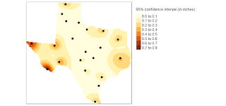
2. Kriging: Kriging is a more advanced interpolation technique that considers both spatial autocorrelation and statistical analysis. It generates a prediction surface by estimating a semivariogram model, which describes the spatial correlation of the data. Kriging provides estimates with optimal accuracy and takes into account the spatial variability and the relationships between the data points. Variants of kriging include ordinary kriging, which assumes a constant mean, and universal kriging, which incorporates a trend component.

3. Radial Basis Functions (RBF): RBF interpolation uses mathematical functions to model the spatial variation between known points. It fits a smooth surface through the data points and evaluates the function at the unknown locations to estimate their values. RBF methods can handle irregularly distributed data points and effectively capture local variations.

4. Natural Neighbor Interpolation: This method calculates the value at an unknown location by considering the proximity of that location to the known points. It creates Voronoi polygons around each known point and uses the area overlap between the unknown location and the polygons to assign weights. Natural neighbor interpolation provides smoother results and avoids abrupt changes between neighboring areas.

5. Spline Interpolation: Splines are mathematical functions that interpolate between known data points to create a smooth surface. They minimize overall curvature and provide a visually appealing result. Spline interpolation can be performed using different approaches such as ordinary splines, tension splines, or B-splines.

6. Trend Surface Analysis: Trend surface analysis examines the trend or pattern present in the data and uses it to estimate values at unknown locations. It fits a polynomial surface to the known points, capturing the general trend and allowing for prediction beyond the data extent. Trend surface analysis can be useful when there is a clear spatial trend or gradient in the data.

These are some commonly used techniques for spatial interpolation in GIS. The choice of method depends on factors such as the nature of the data, the spatial distribution, the desired level of accuracy, and the specific objectives of the analysis. It's important to assess the strengths and limitations of each technique and select the most appropriate method for the given data and analysis requirements.