Raster Analysis

Raster analysis is a powerful spatial analysis technique used in GIS to process and interpret grid-based datasets. It is widely applied in fields such as land cover classification, terrain modeling, hydrological studies, environmental monitoring, and spatial decision-making.

How Raster Analysis Works

Raster data is stored in a grid format where each cell (or pixel) represents a specific geographic location and contains a single value. The value can represent elevation, temperature, land cover type, or any other spatially continuous variable.

1. Spatial Resolution

• The size of each cell in a raster dataset determines the level of detail.
• Example: A 30m resolution DEM (Digital Elevation Model) means each cell represents a 30m × 30m area.

2. Extent

• The geographic area covered by a raster dataset.
• Example: A raster covering an entire country will have a larger extent than one covering a single city.

3. Cell Values and Data Types

• Continuous Data: Represents smoothly varying phenomena (e.g., elevation, temperature, precipitation).
• Categorical (Discrete) Data: Represents distinct classes (e.g., land use types, soil types).

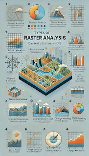
Types of Raster Analysis in GIS

1. Overlay Analysis

Combines multiple raster layers to identify spatial relationships.

• Example: Identifying flood-prone areas by overlaying elevation, rainfall, and land use rasters.

2. Suitability Analysis

Determines the best location for a specific activity based on multiple criteria.

• Example: Finding a suitable site for a wind farm using layers like wind speed, land use, and proximity to roads.

3. Slope Analysis

Calculates the steepness of terrain from a DEM.

• Example: Identifying areas with slopes greater than 30° for landslide risk assessment.

4. Aspect Analysis

Determines the direction a slope is facing.

• Example: Finding south-facing slopes suitable for solar panel installation.

5. Distance Analysis

Measures the distance from a given feature.

• Example: Mapping areas within 1 km of a river for ecological conservation.

6. Zonal Statistics

Summarizes raster values within defined zones (e.g., administrative boundaries).

• Example: Calculating average rainfall within different watersheds.

7. Image Classification

Assigns land cover types to satellite images using supervised or unsupervised classification techniques.

• Example: Classifying Sentinel-2 imagery into urban, forest, water, and agriculture classes.

8. Change Detection

Identifies changes in land cover or other raster datasets over time.

• Example: Analyzing deforestation by comparing Landsat images from 2000 and 2020.

9. Terrain Analysis

Uses DEMs to derive hydrological and topographical features.

• Example: Identifying valleys, ridges, and watershed boundaries.

10. Surface Modeling

Creates interpolated surfaces from point data.

• Example: Generating a temperature surface from scattered weather station data.

Analysis Types Based on Cell Interactions

1. Local Operations (Per-Cell Analysis)

• Each cell is analyzed independently without considering neighbors.
• Example: Applying a mathematical function to all cells in a raster (e.g., converting elevation from meters to feet).

2. Neighborhood Operations (Focal Analysis)

• A cell's value is determined based on surrounding cells.
• Example: Applying a moving window filter (e.g., smoothing an elevation raster using a 3x3 mean filter).

3. Zonal Operations

• Groups of cells belonging to the same zone are analyzed collectively.
• Example: Calculating average elevation within different land use zones.

4. Global Operations

• The entire raster dataset is used to compute an output.
• Example: Calculating flow direction for an entire watershed.